Perceptrons

A motivating example

Perceptrons are a miniature form of neural network and a basic building block of more complex architectures. Before going into the details, let’s motivate them by an example. Assume that we are given a dataset consisting of 100 points in the plane. Half of the points are red and half of the points are blue.

As we can see, the red points are centered at $(-2, -2)$ and the blue points are centered at $(2, 2)$. Now, having seen this data, we can ask ourselves whether there is a way to determine if a point should be red or blue. For example, if someone asks us what the color of the point $(3, 2)$ should be, we’d best respond with blue. Even though this point was not part of the data we have seen, we can infer this since it is located in the blue region of the space.

But what is the general rule to determine if a point is more likely to be blue than red? Apparently, we can draw a line $y = -x$ that nicely separates the space into a red region and a blue region:

We can implicitly represent this line using a weight vector $w$ and a bias $b$. The line then corresponds to the set of points $x$ where

$$w^T x + b = 0.$$

In the case above, we have $w = (1, 1)^T$ and $b = 0$. Now, in order to test whether the point is blue or red, we just have to check whether it is above or below the line. This can be achieved by checking the sign of $w^T x + b$. If it is positive, then $x$ is above the line. If it is negative, then $x$ is below the line. Let’s perform this test for our example point $(3, 2)^T$:

$$
\begin{pmatrix}
1 & 1
\end{pmatrix}
\cdot \begin{pmatrix}
3 \\
2
\end{pmatrix} = 5
$$

Since 5 > 0, we know that the point is above the line and, therefore, should be classified as blue.

Perceptron definition

In general terms, a classifier is a function $\hat{c} : \mathbb{R}^d \rightarrow \{1, 2, …, C\}$ that maps a point onto one of $C$ classes. A binary classifier is a classifier where $C = 2$, i.e. we have two classes. A perceptron with weight $w \in \mathbb{R}^d$ and bias $b \in \mathbb{R}^d$ is a binary classifier where

$$
\hat{c}(x) =
\begin{cases}
1, & \text{if } w^T x + b \geq 0 \\
2, & \text{if } w^T x + b < 0
\end{cases}
$$

$\hat{c}$ partitions $\mathbb{R}^d$ into two half-spaces, each corresponding to one of the two classes. In the 2-dimensional example above, the partitioning is along a line. In general, the partitioning is along a $d-1$ dimensional hyperplane.

From classes to probabilities

Depending on the application, we may be interested not only in determining the most likely class of a point, but also the probability with which it belongs to that class. Note that the higher the value of $w^T x + b$, the higher is its distance to the separating line and, therefore, the higher is our confidence that it belongs to the blue class. But this value can be arbitrarily high. In order to turn this value into a probability, we need to “squash” the values to lie between 0 and 1. One way to do this is by applying the sigmoid function $\sigma$:

$$p(\hat{c}(x) = 1 \mid x) = \sigma(w^T x + b)$$

where $$\sigma(a) = \frac{1}{1 + e^{-a}}$$

Let’s take a look at what the sigmoid function looks like:

As we can see, the sigmoid function assigns a probability of 0.5 to values where $w^T x + b = 0$ (i.e. points on the line) and asymptotes towards 1 the higher the value of $w^T x + b$ becomes, and towards 0 the lower it becomes, which is exactly what we want.

Let’s now define the sigmoid function as an operation, since we’ll need it later:

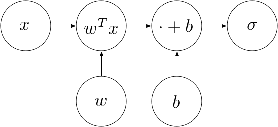
The entire computational graph of the perceptron now looks as follows:

Example

Using what we have learned, we can now build a perceptron for the red/blue example in Python.

Let’s use this perceptron to compute the probability that $(3, 2)^T$ is a blue point:

Multi-class perceptron

So far, we have used the perceptron as a binary classifier, telling us the probability $p$ that a point $x$ belongs to one of two classes. The probability of $x$ belonging to the respective other class is then given by $1-p$. Generally, however, we have more than two classes. For example, when classifying an image, there may be numerous output classes (dog, chair, human, house, …). We can extend the perceptron to compute multiple output probabilities.

Let $C$ denote the number of output classes. We want to perform multiple linear classifications in parallel, one for each of the $C$ classes. To do this, we introduce a weight vector for each class ($w_1, w_2, …, w_C$) and a bias value for each class ($b_1, b_2, …, b_C$). The output of our perceptron should now be a $C$-dimensional vector, each of whose entries contains the probability of the respective class:

$$
output = \left(
\begin{array}{c}
\sigma(w_1^Tx + b_1)\\
\sigma(w_2^Tx + b_2)\\
…\\
\sigma(w_C^Tx + b_C)\\
\end{array}
\right)
$$

In order to do this efficiently, we arrange the weight vectors in a matrix $W = (w_1, w_2, …, w_C) \in \mathbb{R}^{d \times C}$ whose columns correspond to the $w_i$s. Similarly, we arrange the bias values in a vector $b = (b_1, b_2, …, b_C)^T \in \mathbb{R}^C$.

Instead of computing each entry of the output individually, we do the following:

1. Compute $x \cdot W$, which yields the following:
   $$
   \left(
   \begin{array}{c}
   w_1^Tx\\
   w_2^Tx\\
   …\\
   w_C^Tx\\
   \end{array}
   \right)
   $$
2. Add the bias vector $b$, which yields the following:
   $$
   \left(
   \begin{array}{c}
   w_1^Tx + b_1\\
   w_2^Tx + b_2\\
   …\\
   w_C^Tx + b_C\\
   \end{array}
   \right)
   $$
3. Apply the sigmoid element-wise, which yields our intended output:
   $$
   \left(
   \begin{array}{c}
   \sigma(w_1^Tx + b_1)\\
   \sigma(w_2^Tx + b_2)\\
   …\\
   \sigma(w_C^Tx + b_C)\\
   \end{array}
   \right)
   $$

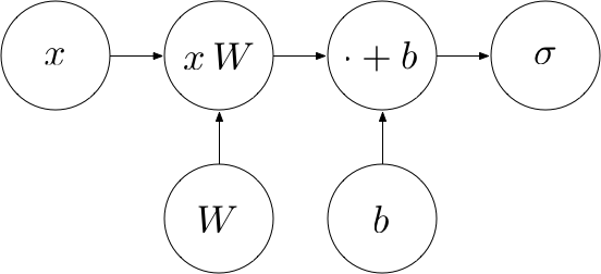
The following computational graph describes this procedure:

Softmax

When the output classes are disjoint, the output probabilities should sum up to one. In this case, we apply the softmax function to the vector $a = xW + b$ instead of the element-wise sigmoid, which makes sure that each probability is between 0 and 1 and the sum of the probabilities is 1:

$$
\sigma(a)_i = \frac{e^{a_i}}{\sum_{j = 1}^C e^{a_j}}
$$

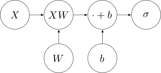
Batch computation

The matrix form allows us to feed in more than one point at a time. That is, instead of a single point $x$, we could feed in a matrix $X \in \mathbb{R}^{N \times d}$ containing one point per row (i.e. $N$ rows of $d$-dimensional points). We refer to such a matrix as a batch. Instead of $xW$, we compute $XW$. This returns an $N \times C$ matrix, each of whose rows contains $xW$ for one point $x$. To each row, we add a bias vector $b$, which is now an $1 \times m$ row vector. The whole procedure thus computes a function $f : \mathbb{R}^{N \times d} \rightarrow \mathbb{R}^{m}$ where $f(X) = \sigma(XW + b)$. The computational graph looks as follows:

Example

Let’s now generalize our red/blue perceptron to allow for batch computation and multiple output classes.

Since the first 10 points in our data are all blue, the perceptron outputs high probabilities for blue (left column) and low probabilities for red (right column), as expected.