This is part 1 of a series of tutorials, in which we develop the mathematical and algorithmic underpinnings of deep neural networks from scratch and implement our own neural network library in Python, mimicing the TensorFlow API.
- Part I: Computational Graphs
- Part II: Perceptrons
- Part III: Training criterion
- Part IV: Gradient Descent and Backpropagation
- Part V: Multi-Layer Perceptrons
- Part VI: TensorFlow
I do not assume that you have any preknowledge about machine learning or neural networks. However, you should have some preknowledge of calculus, linear algebra, fundamental algorithms and probability theory on an undergraduate level. If you get stuck at some point, please leave a comment.
By the end of this text, you will have a deep understanding of the math behind neural networks and how deep learning libraries work under the hood.
I have tried to keep the code as simple and concise as possible, favoring conceptual clarity over efficiency. Since our API mimics the TensorFlow API, you will know how to use TensorFlow once you have finished this text, and you will know how TensorFlow works under the hood conceptually (without all the overhead that comes with an omnipotent, maximally efficient machine learning API).
The full source code of the API can be found at https://github.com/danielsabinasz/TensorSlow. You also find a Jupyter Notebook there, which is equivalent to this blog post but allows you to fiddle with the code.
Computational graphs
We shall start by defining the concept of a computational graph, since neural networks are a special form thereof. A computational graph is a directed graph where the nodes correspond to operations or variables. Variables can feed their value into operations, and operations can feed their output into other operations. This way, every node in the graph defines a function of the variables.
The values that are fed into the nodes and come out of the nodes are called tensors, which is just a fancy word for a multi-dimensional array. Hence, it subsumes scalars, vectors and matrices as well as tensors of a higher rank.
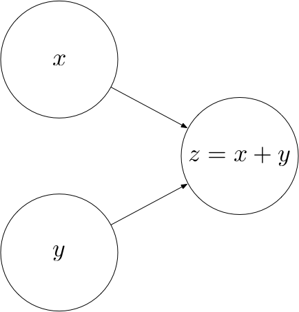
Let’s look at an example. The following computational graph computes the sum $z$ of two inputs $x$ and $y$.
Here, $x$ and $y$ are input nodes to $z$ and $z$ is a consumer of $x$ and $y$. $z$ therefore defines a function $z : \mathbb{R^2} \rightarrow \mathbb{R}$ where $z(x, y) = x + y$.

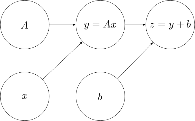
The concept of a computational graph becomes more useful once the computations become more complex. For example, the following computational graph defines an affine transformation $z(A, x, b) = Ax + b$.

Operations
Every operation is characterized by three things:
- A
computefunction that computes the operation’s output given values for the operation’s inputs - A list of
input_nodeswhich can be variables or other operations - A list of
consumersthat use the operation’s output as their input
Let’s put this into code:
Some elementary operations
Let’s implement some elementary operations in order to become familiar with the Operation class (and because we will need them later). In both of these operations, we assume that the tensors are NumPy arrays, in which the element-wise addition and matrix multiplication (.dot) are already implemented for us.
Addition
Matrix multiplication
Placeholders
Not all the nodes in a computational graph are operations. For example, in the affine transformation graph, $A$, $x$ and $b$ are not operations. Rather, they are inputs to the graph that have to be supplied with a value once we want to compute the output of the graph. To provide such values, we introduce placeholders.
Variables
In the affine transformation graph, there is a qualitative difference between $x$ on the one hand and $A$ and $b$ on the other hand. While $x$ is an input to the operation, $A$ and $b$ are parameters of the operation, i.e. they are intrinsic to the graph. We will refer to such parameters as Variables.
The Graph class
Finally, we’ll need a class that bundles all the operations, placeholders and variables together. When creating a new graph, we can call its as_default method to set the _default_graph to this graph. This way, we can create operations, placeholders and variables without having to pass in a reference to the graph everytime.
Example
Let’s now use the classes we have built to create a computational graph for the following affine transformation:
$$
z = \begin{pmatrix}
1 & 0 \\
0 & -1
\end{pmatrix}
\cdot
x
+
\begin{pmatrix}
1 \\
1
\end{pmatrix}
$$
Computing the output of an operation
Now that we are confident creating computational graphs, we can start to think about how to compute the output of an operation.
Let’s create a Session class that encapsulates an execution of an operation. We would like to be able to create a session instance and call a run method on this instance, passing the operation that we want to compute and a dictionary containing values for the placeholders:
session = Session()
output = session.run(z, {
    x: [1, 2]
})
This should compute the following value:
$$
z = \begin{pmatrix}
1 & 0 \\
0 & -1
\end{pmatrix}
\cdot
\begin{pmatrix}
1 \\
2
\end{pmatrix}
+
\begin{pmatrix}
1 \\
1
\end{pmatrix}
=
\begin{pmatrix}
2 \\
-1
\end{pmatrix}
$$
In order to compute the function represented by an operation, we need to apply the computations in the right order. For example, we cannot compute $z$ before we have computed $y$ as an intermediate result. Therefore, we have to make sure that the operations are carried out in the right order, such that the values of every node that is an input to an operation $o$ has been computed before $o$ is computed. This can be achieved via post-order traversal.
Let’s test our class on the example from above:
Looks good.
If you have any questions, feel free to leave a comment. Otherwise, continue with the next part: II: Perceptrons.


This is the website I’ve been looking for for months. Really, really nicely done. Thanks!
Where is `dot()` coming from?
We assume that our multi-dimensional data are numpy arrays, which have such a dot function. I’ll try to incorporate that into the text.
Where is operation.output defined?
In the Session.run method, we iterate over all nodes in order and set their output (node.output). “operation” is one of these nodes, so after the loop we know that its output has been set and we can return it.
Excellent blogs! Can I translate your blog into Chinese? Of course I will keep your original blog URL. 🙂
I’d very much welcome a translation. However, please do not create a Chinese copy of the website under the same name (like deepideas.cn). If you send me your translations, I can post them as translations to sabinasz.net in your name. Or, if you prefer, you could post them on your own personal blog and link back to the original version.
When i try to compile the code i am getting error “NameError: name ‘add’ is not defined”
can someone tell me what i am missing
thanks.
sorry, i missed the definition off add in a code. Had matmul though 🙂
So please ignore question.
Daniel, that is a really good blog post. Really in line with what I was looking for.
I implemented your code, but I got a error. I tried to debug the code, but I did not have much luck:
AttributeError: ‘add’ object has no attribute ‘output’
any ideas of why phyton is returning this error?
Hi Victor,
when I copy paste the whole code into one file, it works for me. Can you send me your whole code so I can run it?
Best,
Daniel
Have the following error: ‘Variable’ object has no attribute ‘dot’
for both hand-copied and direct-copied code (into a single file)
Any ideas?
It is hard to guess without the code. But if you only implemented the the code in the part I, there is no dot operation defined here. Only matmul and addition. Your code is probably calling dot somewhere, but is was indeed not defined.
Apologies, forgot to include detailed error message, was done late at night 🙂
Fixed now anyway, not quite sure what the issue was but was related to calling the a.dot(b) function.
Anyone else thinking that the notepads might have hidden scripts/imports – they don’t, have faith in the code aha.
# Iterate all nodes to determine their value
for node in nodes_postorder:
if type(node) == placeholder:
# Set the node value to the placeholder value from feed_dict
node.output = feed_dict[node]
elif type(node) == Variable:
# Set the node value to the variable’s value attribute
node.output = node.value
else: # Operation
# Get the input values for this operation from node_values
node.inputs = [input_node.output for input_node in node.input_nodes]
# Compute the output of this operation
node.output = node.compute(*node.inputs)
# Convert lists to numpy arrays
if type(node.output) == list:
node.output = np.array(node.output)
# Return the requested node value
return operation.output
Precisely, what are “.inputs” & “.output” from Python perspective?
Question 1:
Can we say placeholders contain variables as a set? Or these two are seperated from each other?
While A and b are variables, x is a placeholder. According to the definition, any computational graph has to be consisted of operations or variables. How about placeholders? It seems to me that you also said that placeholders and variables are different:
“In the affine transformation graph, there is a qualitative difference between x on the one hand and A and b on the other hand. “
Placeholders are in this graph too. Should we change the definition of computatinal graph from “… correspon to operations or variables” to “… correspond to operations or inputs”, since you call inputs both variables and placeholders:
“A, x and b are not operations. Rather, they are inputs to the graph that have to be supplied with a value once we want to compute the output of the graph.”
Actually, there is another statement that you made , which is
“While x is an input to the operation, A and b are parameters of the operation, i.e. they are intrinsic to the graph.”
It seems inputs dont contain both placeholders and variables.
Summary: There is a confusion for me here. I hope you will take care of it by explaning following keywords in more detail once for me: Input, variable, placeholder, parameter.
Question 2:
About tensors… Does a tensor have to provide the following two conditions?
-: values that are fed into the nodes
–: values that are come out of the nodes.
Cant we define A, x, Z tensor, while we can y? Or… We can define all these nodes in the graph as a tensor?
Thank you for this very nice tutorial!
It’s useful. Thank you very much!